Feature extraction and spatial analysis

This notebook demonstrates a powerful, annotation-free workflow for analyzing the morphological landscape of a Whole Slide Image (WSI). The core idea is to leverage a pre-trained deep learning model to automatically extract meaningful features from image tiles and then use standard clustering tools to cluster and visualize these features.

The process involves three main steps:

• Tiling.

• Feature Extraction: A pre-trained vision model is used to process each tile. The model converts the visual information of each patch into a high-dimensional feature vector—a numerical signature that represents its content.

• Downstream Analysis: These feature vectors are then analyzed using a pipeline common in single-cell genomics. We will perform dimensionality reduction with PCA, build a neighborhood graph, and then use UMAP for visualization and the Leiden algorithm for clustering.

By the end of this workflow, we will have generated a UMAP embedding that visually organizes the tiles by similarity and a clustered map of the tiles of the WSI, effectively segmenting the tissue into distinct morphological regions without any manual intervention.

First, we will load a GTEx Small Intestine slide as example.

from huggingface_hub import hf_hub_download

slide = hf_hub_download(
    "rendeirolab/lazyslide-data",
    "GTEX-11DXX-1626.svs",
    repo_type="dataset",
    cache_dir=".",
)

from wsidata import open_wsi
import lazyslide as zs

Let’s open the wsi!

wsi = open_wsi(slide)
wsi

WSI: datasets--rendeirolab--lazyslide-data/snapshots/c455e26e8fbadada072d2ce348f563fa72c27eb6/GTEX-11DXX-1626.svs
Reader: openslide
Dimensions: 38717×51791 (h×w), 3 Pyramids
Pixel physical size: 0.49 MPP (20X)

SpatialData object
└── Images
      └── 'wsi_thumbnail': DataArray[cyx] (3, 1118, 1495)
with coordinate systems:
    ▸ 'global', with elements:
        wsi_thumbnail (Images)

What does the tissue look like?

zs.pl.tissue(wsi)

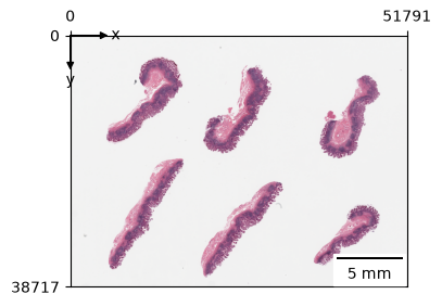
Let’s first find and tile the tissue, we will request tiny tile size of 64*64 px, this may take a while.

zs.pp.find_tissues(wsi)
zs.pp.tile_tissues(wsi, 128)

Morphological feature extraction

Feature extraction is to transform the image into a the numeric representation, which comprises of different morphological features. Typically, this is done by feeding the tiles into a vision model.

LazySlide supports automatic mix-precision inference which may reduce memory usuage and have faster inference spped, try amp=True. Since we are working on a big slide with tiny tile sizes, this may take 10mins to finish (MacBook M3 Max).

zs.tl.feature_extraction(wsi, "plip", amp=True)

::{note} Autocast doesn’t work well with mps backend though, you may get all nan results.

zs.tl.feature_extraction(wsi, "plip")

Features are saved as AnnData store with a convention of “{model name}_{tiles key}”. For example, h0-mini_tiles

Feature aggregation

To perform analysis across dataset, a usual way is to pool features into a 1D vector that can represent the entire slide. By default, the mean pooling is applied. Advanced slide encoders will be introduced later.

zs.tl.feature_aggregation(wsi, feature_key="plip")

You can retrieve specific feature with the fetch accessor. This will return a copy of the anndata.

adata = wsi.fetch.features_anndata("plip")

Pre-computed results

If you don’t want to run feature extraction, you can simply load the pre-computed one

wsi = zs.datasets.gtex_small_intestine()

wsi

Examination of feature space

You may need to install scanpy and igraph to run the following command.

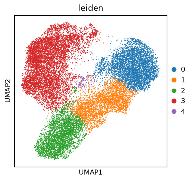
This code takes the deep-learning feature data from image tiles we have extracted from PLIP, preprocesses it, and then performs a standard analysis workflow to identify groups of similar tiles (clustering). We can visualize the tile space using UMAP. The colors represent the different clusters, as found by computing Leiden clustering on the neighborhood graph of tiles.

import scanpy as sc

adata = wsi["plip_tiles"]
sc.pp.scale(adata)
sc.pp.pca(adata)
sc.pp.neighbors(adata)
sc.tl.umap(adata)
sc.tl.leiden(adata, flavor="igraph", resolution=0.2)

sc.pl.umap(adata, color="leiden")

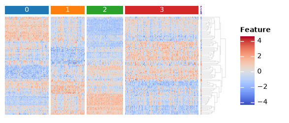
sc.tl.rank_genes_groups(adata, groupby="leiden")

features = set()
for i in adata.obs["leiden"].unique():
    names = sc.get.rank_genes_groups_df(adata, i).names
    features.update(list(names[0:10]) + list(names[-10:]))
features = list(features)

import marsilea as ma
import marsilea.plotter as mp
from scipy.stats import zscore

key = "leiden"
h = ma.Heatmap(zscore(adata[:, features].X.T), height=2, width=4, label="Feature")
order = sorted(adata.obs[key].unique())
h.group_cols(adata.obs[key], order=order)
h.add_top(mp.Chunk(order, fill_colors=adata.uns[f"{key}_colors"], padding=2), pad=0.05)
h.add_dendrogram("right", method="average", linewidth=0.1)
h.add_legends()
h.render()

Identification of spatial domains

The Leiden clustering on features from the foundational model can already recover the spatial domains of tissues pretty well. However, this clustering algorithm is based on the proximity of the morphological features of each tile, but it does not consider actual spatial information.

zs.pl.tiles(
    wsi,
    feature_key="plip",
    color="leiden",
    alpha=0.5,
    palette=adata.uns[f"{key}_colors"],
    show_contours=False,
)

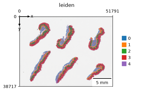
For simplicity, you can run spatial domain analysis with zs.tl.spatial_domain. This is equivalent to the previous analysis.

zs.tl.spatial_domain(wsi, feature_key="plip", resolution=0.2)

wsi.write()

Integration of spatial information with UTAG

In this example, you may notice the border of domain is not very smooth, this can be improved by integrating spatial information.

UTAG is a method develop to discovery spatial domain with unsupervised learning.

The basic idea is to use message passing to combine the physical position of the tiles and the features of each tile to create a spatially-informed neighborhood graph. In the following code block, we first create an adjacency matrix of the tile locations with zs.pp.tile_graph and then integrate spatial tile context with vision features using spatial feature smoothing with zs.tl.spatial_features.

zs.pp.tile_graph(wsi)
zs.tl.spatial_features(wsi, "plip")

zs.tl.spatial_domain(wsi, layer="spatial_features", feature_key="plip", resolution=0.2)

zs.pl.tiles(wsi, color="domain", alpha=0.5)

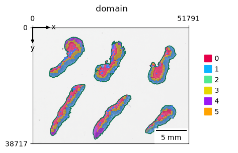
Now we can observe there are 6 domains in the tissues, with smooth borders.

Text feature extraction

Apart from deriving morphological features from vision models, you can also run multimodal to derive text features.

Currently, there are two vision-language models for pathology

• PLIP, Nature Medicine, 2023

• CONCH, Nature Medicine, 2024

Since we’ve extracted the plip vision features for our WSI, we only need to extract features for the texts.

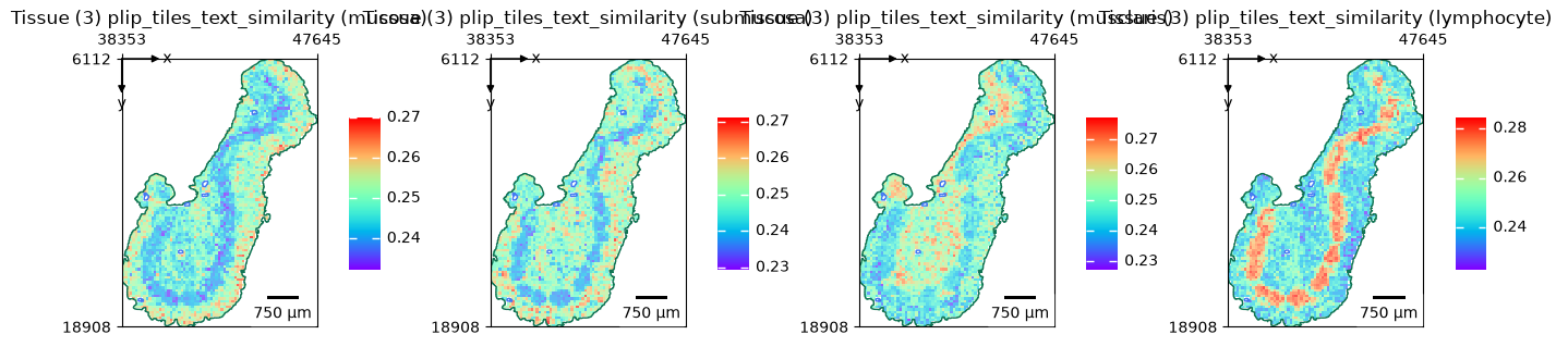
terms = ["mucosa", "submucosa", "musclaris", "lymphocyte"]

embeddings = zs.tl.text_embedding(terms, model="plip")
zs.tl.text_image_similarity(wsi, embeddings, model="plip", softmax=True)

zs.pl.tiles(
    wsi,
    feature_key="plip_tiles_text_similarity",
    color=terms,
    cmap="rainbow",
    show_image=False,
    tissue_id=3,
    alpha=0.7,
)