
Virtual Staining: Zero-Cost Multiplexed Imaging from H&E Images#
This tutorial introduces one of the advanced features of LazySlide: the ability to transform a standard H&E (Hematoxylin and Eosin) histology image into a multiplexed image with multiple predicted biomarker channels. This powerful technique enables researchers to extract rich molecular information from routine histological slides without the need for expensive immunohistochemistry or specialized staining protocols.
# Import LazySlide and load a sample whole slide image (WSI)
import lazyslide as zs

wsi = zs.datasets.sample()
wsi

Reader: openslide
Dimensions: 2967×2220 (h×w), 1 Pyramid
Pixel physical size: 0.50 MPP (20X)
SpatialData object, with associated Zarr store: /home/runner/work/lazyslide-tutorials/lazyslide-tutorials/.cache/huggingface/hub/datasets--RendeiroLab--LazySlide-data/snapshots/d469afd4a763ad366861e8c49d4cf424bfad902c/sample.zarr
├── Shapes
│     ├── 'annotations': GeoDataFrame shape: (3, 4) (2D shapes)
│     ├── 'dl-tissue': GeoDataFrame shape: (2, 2) (2D shapes)
│     ├── 'tiles': GeoDataFrame shape: (31, 3) (2D shapes)
│     └── 'tissues': GeoDataFrame shape: (1, 2) (2D shapes)
└── Tables
      └── 'resnet50_tiles': AnnData (31, 2048)
with coordinate systems:
    ▸ 'global', with elements:
        annotations (Shapes), dl-tissue (Shapes), tiles (Shapes), tissues (Shapes)
zs.pl.tissue(wsi)
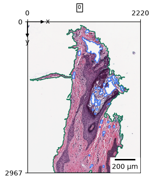
zs.pp.tile_tissues(wsi, 256, stride_px=32)

# Apply virtual staining using the GigaTime model
zs.tl.virtual_stain(wsi, model="gigatime")
Examining the Results#
Let’s examine our WSI object to see how the virtual staining has enhanced our data:
wsi
Reader: openslide
Dimensions: 2967×2220 (h×w), 1 Pyramid
Pixel physical size: 0.50 MPP (20X)
SpatialData object, with associated Zarr store: /home/runner/work/lazyslide-tutorials/lazyslide-tutorials/.cache/huggingface/hub/datasets--RendeiroLab--LazySlide-data/snapshots/d469afd4a763ad366861e8c49d4cf424bfad902c/sample.zarr
├── Images
│     └── 'gigatime_prediction': DataArray[cyx] (23, 2967, 2220)
├── Shapes
│     ├── 'annotations': GeoDataFrame shape: (3, 4) (2D shapes)
│     ├── 'dl-tissue': GeoDataFrame shape: (2, 2) (2D shapes)
│     ├── 'tiles': GeoDataFrame shape: (1776, 3) (2D shapes)
│     └── 'tissues': GeoDataFrame shape: (1, 2) (2D shapes)
└── Tables
      └── 'resnet50_tiles': AnnData (31, 2048)
with coordinate systems:
    ▸ 'global', with elements:
        gigatime_prediction (Images), annotations (Shapes), dl-tissue (Shapes), tiles (Shapes), tissues (Shapes)
with the following elements not in the Zarr store:
    ▸ gigatime_prediction (Images)
Understanding Virtual Staining Output#
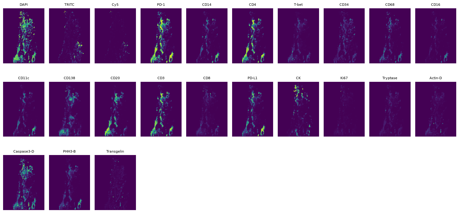
The virtual staining process generates predicted biomarker images that are stored in the images slot of the WSI data object (SpatialData format).
ROSIE
The ROSIE model makes predictions at the tile level, generating a mean expression value for each biomarker within each tile
This approach provides spatial gene expression predictions across the entire tissue section
For higher resolution results, consider using smaller tile sizes with more overlap
To replicate the exact settings from the original ROSIE paper, use:
zs.pp.tile_tissues(wsi, 128, stride_px=8)
GigaTIME
If you use GigaTIME model, it’s a UNet structure model that predict the pixel level expression.
Let’s explore the generated predictions:
# Access the virtual staining predictions stored in the images dictionary
wsi.images["gigatime_prediction"]
<xarray.DataArray 'image' (c: 23, y: 2967, x: 2220)> Size: 606MB
dask.array<array, shape=(23, 2967, 2220), dtype=float32, chunksize=(23, 1207, 1207), chunktype=numpy.ndarray>
Coordinates:
  * c        (c) <U10 920B 'DAPI' 'TRITC' 'Cy5' ... 'PHH3-B' 'Transgelin'
  * y        (y) float64 24kB 0.5 1.5 2.5 3.5 ... 2.964e+03 2.966e+03 2.966e+03
  * x        (x) float64 18kB 0.5 1.5 2.5 3.5 ... 2.218e+03 2.218e+03 2.22e+03
Attributes:
transform: {'global': Scale (y, x)\n [1. 1.]}# Display all available biomarker channels predicted by the GigaTime model
wsi.images["gigatime_prediction"].c.data
array(['DAPI', 'TRITC', 'Cy5', 'PD-1', 'CD14', 'CD4', 'T-bet', 'CD34', 'CD68',
       'CD16', 'CD11c', 'CD138', 'CD20', 'CD3', 'CD8', 'PD-L1', 'CK', 'Ki67',
       'Tryptase', 'Actin-D', 'Caspase3-D', 'PHH3-B', 'Transgelin'],
      dtype='<U10')
# Visualize all predicted biomarker channels in a grid layout
import matplotlib.pyplot as plt

# Create a 5x10 subplot grid to display all 50 biomarker channels
n_markers = wsi.images["gigatime_prediction"].data.shape[0]
n_cols = 10
n_rows = (n_markers + n_cols - 1) // n_cols  # Calculate number of rows needed
fig, axs = plt.subplots(n_rows, n_cols, figsize=(15, 2.5 * n_rows))
axs = axs.flatten()

# Plot each biomarker channel with its corresponding gene name as title
for i in range(n_markers):
    ax = axs[i]
    ax.imshow(wsi.images["gigatime_prediction"].data[i])
    ax.set_title(wsi.images["gigatime_prediction"].c.data[i], fontsize=8)
    ax.axis("off")

# Turn off any unused subplots
for j in range(i + 1, n_rows * n_cols):
    axs.flatten()[j].axis("off")

plt.tight_layout()
plt.show()
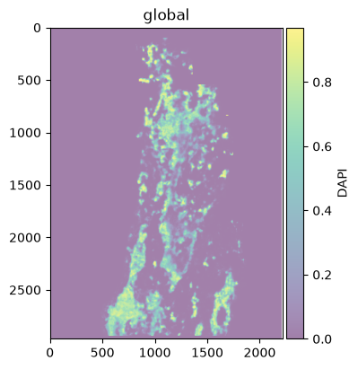
You can also use spatialdata plot to overlay specific biomarker channels on the original H&E image for better visualization.
import spatialdata_plot  # noqa: F401

(wsi.pl.render_images("gigatime_prediction", channel=["DAPI"], alpha=0.5).pl.show())
Summary#
Congratulations! You’ve successfully applied virtual staining to transform a standard H&E image into a rich, multiplexed dataset. This technique opens up numerous possibilities for:
Biomarker discovery: Identify spatial patterns of gene expression without expensive assays
Digital pathology: Enhance routine histological analysis with molecular insights
Research acceleration: Generate hypotheses about tissue biology from existing slide archives
Cost-effective screening: Prioritize samples for expensive molecular assays
The virtual staining approach represents a powerful bridge between traditional histopathology and modern molecular biology, enabling researchers to extract maximum value from standard histological preparations.