Preprocessing a WSI: From raw image to analysis-ready data

Preprocessing a WSI: From raw image to analysis-ready data#

Welcome to the second tutorial in our LazySlide series! In this lesson, we’ll walk you through a complete workflow for preprocessing whole slide images (WSIs). Preprocessing is a crucial step that transforms raw WSI data into a format that’s ready for advanced analysis.

By the end of this tutorial, you’ll understand how to:

Load and examine WSI data
Segment tissue regions from the background
Evaluate tissue quality
Create tiles (smaller patches) from large WSIs
Extract meaningful features from these tiles

Let’s get started with this essential foundation for computational pathology!

Setting up environment#

Let’s start by importing the LazySlide library. Throughout all our tutorials, we’ll use the convention of importing LazySlide as zs - this makes our code consistent and easy to read. This naming convention is similar to how other popular libraries like pandas (pd) and numpy (np) are typically imported.

import lazyslide as zs

Step 1: Opening a whole slide image#

Our first task is to load a whole slide image for processing. For this tutorial, we’ll download a sample artery tissue slide from the GTEx project. This is the same slide we explored in the previous tutorial, so you should already be familiar with its basic structure.

from huggingface_hub import hf_hub_download

slide = hf_hub_download(
    "rendeirolab/lazyslide-data", 
    "GTEX-1117F-0526.svs", 
    repo_type="dataset",
    cache_dir="."
)

Step 2: Understanding the WSIData object#

A key concept in LazySlide is the WSIData object, which is the foundation of our analysis workflow. Let’s take a moment to understand what makes this object so powerful:

WSIData extends the SpatialData framework, adding specialized capabilities for working with whole slide images
It provides a unified interface for accessing both the image data and associated metadata regardless of your WSI format
It’s compatible with other packages in the scverse ecosystem, allowing for seamless integration with single-cell analysis tools
It maintains a connection to your original WSI file while storing analysis results separately

When you open a WSI, the system automatically creates a WSIData object. By default, this object is stored in a directory alongside your original WSI file, making it easy to find and reuse your analysis results later.

If you’re interested in learning more about the technical details, you can explore the WSIData documentation.

Now, let’s create our WSIData object:

from wsidata import open_wsi

wsi = open_wsi(slide)

Step 3: Exploring WSIData object#

Let’s examine what’s inside our newly created WSIData object. This will help us understand the structure and components that we’ll be working with throughout our analysis.

wsi

WSI: datasets--rendeirolab--lazyslide-data/snapshots/c455e26e8fbadada072d2ce348f563fa72c27eb6/GTEX-1117F-0526.svs
Reader: openslide
Dimensions: 19958×19919 (h×w), 3 Pyramids
Pixel physical size: 0.49 MPP (20X)

SpatialData object
└── Images
      └── 'wsi_thumbnail': DataArray[cyx] (3, 1996, 1992)
with coordinate systems:
    ▸ 'global', with elements:
        wsi_thumbnail (Images)

Now, let’s look at the important metadata of our slide. This information tells us crucial details about how the slide was scanned and its dimensions. For example, we can see that this slide was scanned at 20X magnification with a resolution of 0.4942 microns per pixel (mpp). We can also see that the full-resolution image has dimensions of 19958×19919 pixels - that’s nearly 400 million pixels in total!

wsi.properties

Slide Properties

Field	Value
shape	[19958, 19919]
n_level	3
level_shape	[[19958, 19919], [4989, 4979], [2494, 2489]]
level_downsample	[1.0, 4.000501706284455, 8.002609074152414]
mpp	0.4942
magnification	20.0
bounds	[0, 0, 19919, 19958]

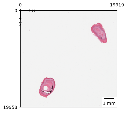
Let’s visualize our slide to get a better understanding of what we’re working with. LazySlide makes it easy to render a whole slide image with just a single line of code using the tissue function from the plotting module.

zs.pl.tissue(wsi)

../_images/c9669a02783ccd1775cc490cf0302899881c05b8c8bd00c48a22cd067ce915ea.png

Saving Our Work#

An important aspect of working with WSIData is that all changes are initially stored in memory. To preserve our work between sessions, we need to save it to disk. This can be done easily with the .write() method. By default, this saves our WSIData in a directory right next to our original slide file. This will not only make it easier for you to locate the store but it will also be automatically picked up when you open a WSI.

wsi.write()

Step 4: Tissue Segmentation#

One of the most fundamental steps in WSI analysis is tissue segmentation - the process of identifying and isolating the actual tissue regions from the background and artifacts. This step is crucial because:

It reduces the computational burden by focusing only on relevant areas
It eliminates background areas that could introduce noise into our analysis
It allows us to work with distinct tissue pieces separately

LazySlide provides powerful tools to automatically detect tissue regions. Let’s see how this works:

zs.pp.find_tissues(wsi)

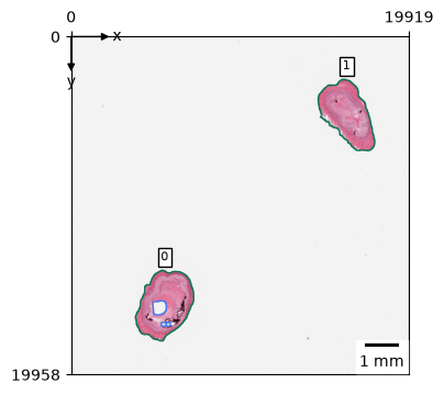
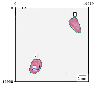
Let’s visualize the results of our tissue segmentation to make sure it worked correctly. In the visualization:

The green lines show the borders of detected tissue regions
The blue areas represent holes or empty spaces within the tissue that will be excluded from analysis

The default parameters of the tissue segmentation algorithm usually work quite well for most slides, but LazySlide offers many options to fine-tune the segmentation if needed.

zs.pl.tissue(wsi)

../_images/16f1c39c1d3cde1aed48948dd951a6317973e79c2e08fc07f15c5b862e170fda.png

Examining the segmentation results#

If we examine our WSIData object again, we’ll notice something new: a GeoDataFrame named tissues has been added to the Shapes slot in our SpatialData object. This is where LazySlide stores the geometric information about each tissue region we’ve identified.

wsi

WSI: datasets--rendeirolab--lazyslide-data/snapshots/c455e26e8fbadada072d2ce348f563fa72c27eb6/GTEX-1117F-0526.svs
Reader: openslide
Dimensions: 19958×19919 (h×w), 3 Pyramids
Pixel physical size: 0.49 MPP (20X)

SpatialData object, with associated Zarr store: /home/runner/work/lazyslide-tutorials/lazyslide-tutorials/tutorials/datasets--rendeirolab--lazyslide-data/snapshots/c455e26e8fbadada072d2ce348f563fa72c27eb6/GTEX-1117F-0526.zarr
├── Images
│     └── 'wsi_thumbnail': DataArray[cyx] (3, 1996, 1992)
└── Shapes
      └── 'tissues': GeoDataFrame shape: (2, 2) (2D shapes)
with coordinate systems:
    ▸ 'global', with elements:
        wsi_thumbnail (Images), tissues (Shapes)
with the following elements not in the Zarr store:
    ▸ tissues (Shapes)

We can access this table using dictionary-style notation with the key “tissues”. Let’s take a look at what information is stored for each tissue region.

Each row in this table represents a distinct tissue piece, and each tissue is assigned a unique tissue_id. This identifier is extremely useful as it allows us to:

Reference specific tissue pieces in our analysis
Track tissue pieces across different processing steps
Apply operations to individual tissues rather than the entire slide

You might have noticed that these tissue_id values were also displayed in our earlier visualization, making it easy to connect visual information with the data in our tables.

wsi["tissues"]

	tissue_id	geometry
0	0	POLYGON ((5345.743 13804.501, 5337.74 13812.50...
1	1	POLYGON ((16029.226 2520.822, 16021.223 2528.8...

Focusing on individual tissue pieces#

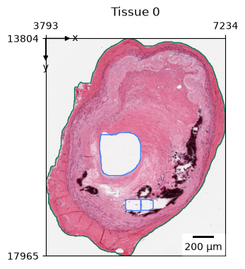
One of the advantages of tissue segmentation is the ability to focus on specific regions of interest. LazySlide makes it easy to zoom in on a particular tissue piece by specifying its tissue_id in the visualization function. This is particularly useful when working with slides that contain multiple distinct tissue sections.

zs.pl.tissue(wsi, tissue_id=0)

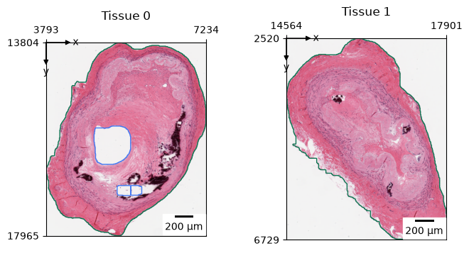
../_images/e7ab5ec9526acae560048d6f01f2249faeb8d1ef0bef098aa85baa0ab529e301.png

You may also show all tissue pieces at once by specifying tissue_id="all"

zs.pl.tissue(wsi, tissue_id="all")

../_images/d044f0e0c9147d11fa849d1d74c412d68cb127edbdd7172e5ee80fd918d5efae.png

Don’t forget to save your work!#

Remember that all the processing we’ve done so far (tissue segmentation, etc.) is stored in memory until we explicitly save it. It’s a good practice to save your work periodically, especially after completing important processing steps. This ensures you won’t lose your progress if your session ends unexpectedly.

wsi.write()

Loading previously saved work#

One of the great benefits of saving your work is that you can easily pick up where you left off in a future session. LazySlide automatically looks for existing WSIData when you open a slide, making it seamless to continue your analysis:

wsi = open_wsi(slide)

Advanced topic: Deep learning-based tissue segmentation#

In addition to the traditional image processing techniques we’ve used so far, LazySlide also offers more advanced deep learning-based approaches to tissue segmentation.

Let’s try the deep learning-based segmentation approach:

zs.seg.tissue(wsi, key_added="dl-tissues")

wsi

WSI: datasets--rendeirolab--lazyslide-data/snapshots/c455e26e8fbadada072d2ce348f563fa72c27eb6/GTEX-1117F-0526.svs
Reader: openslide
Dimensions: 19958×19919 (h×w), 3 Pyramids
Pixel physical size: 0.49 MPP (20X)

SpatialData object, with associated Zarr store: /home/runner/work/lazyslide-tutorials/lazyslide-tutorials/tutorials/datasets--rendeirolab--lazyslide-data/snapshots/c455e26e8fbadada072d2ce348f563fa72c27eb6/GTEX-1117F-0526.zarr
├── Images
│     └── 'wsi_thumbnail': DataArray[cyx] (3, 1996, 1992)
└── Shapes
      ├── 'dl-tissues': GeoDataFrame shape: (2, 2) (2D shapes)
      └── 'tissues': GeoDataFrame shape: (2, 2) (2D shapes)
with coordinate systems:
    ▸ 'global', with elements:
        wsi_thumbnail (Images), dl-tissues (Shapes), tissues (Shapes)
with the following elements not in the Zarr store:
    ▸ dl-tissues (Shapes)

zs.pl.tissue(wsi, tissue_key="dl-tissues")

../_images/9b28f8b5871d56b1e234c29fd4abe3ed5c9cff7c32d1bbba2d2764d6824a7c19.png

Calculating tissue properties#

Beyond just identifying tissue regions, it’s often valuable to calculate various geometric properties of each tissue piece. These properties can provide insights into tissue morphology and can be used as features in downstream analysis.

LazySlide makes it easy to calculate a comprehensive set of geometric properties for each tissue instance, including:

Area and perimeter
Compactness and roundness
Major and minor axis lengths
Orientation and eccentricity

Let’s calculate these properties for our tissue pieces:

zs.tl.tissue_props(wsi)

wsi["tissues"]

	tissue_id	geometry	area	area_filled	convex_area	solidity	convexity	axis_major_length	axis_minor_length	eccentricity	...	moment-mu21	moment-mu12	moment-mu03	moment-nu20	moment-nu11	moment-nu02	moment-nu30	moment-nu21	moment-nu12	moment-nu03
0	0	POLYGON ((5345.743 13804.501, 5337.74 13812.50...	9295453.0	9962045.0	10318845.0	0.900823	1.110096	4348.672363	2953.654297	0.733946	...	1.881723e+14	-5.012970e+14	6.182167e+13	0.068301	-0.026006	0.104072	0.000592	0.000601	-0.001600	0.000197
1	1	POLYGON ((16029.226 2520.822, 16021.223 2528.8...	8684173.0	8684173.0	9086193.5	0.955755	1.046293	4684.261719	2505.699219	0.844904	...	6.244954e+14	1.792367e+15	1.164329e+15	0.074724	0.048856	0.123623	-0.002956	0.002810	0.008065	0.005239

2 rows × 51 columns

Step 5: Tiling - Breaking down the WSI into manageable pieces#

We’ve now reached one of the most important preprocessing steps: tiling (also called patching). This process involves dividing the large whole slide image into smaller, manageable pieces that can be processed individually.

Why tiling is essential#

Tiling solves several critical challenges in WSI analysis:

Memory constraints: As we’ve discussed, whole slide images are enormous (often several GB) and cannot fit entirely into memory
Computational efficiency: Working with smaller tiles allows for parallel processing and faster analysis
Feature extraction: Most deep learning models expect inputs of a fixed size, making tiles ideal for feature extraction
Localized analysis: Tiling preserves spatial information while allowing for detailed analysis of specific regions

Harmonization Across Slides#

Note

When working with multiple slides from different sources, harmonization becomes crucial to account for batch effects. If your slides were scanned at different magnifications, you should specify a consistent microns-per-pixel (mpp) value during tiling to ensure all tiles represent the same physical area, regardless of the original scanning resolution.

Here is a list of mpp value map with magnification:

Magnification	MPP (Microns per Pixel)
40×	0.25
20×	0.5
10×	1

These values are approximate and may vary depending on the scanner, so check the specifications of magnification and resolution on the slide metadata!

LazySlide’s flexible tiling capabilities#

LazySlide offers exceptional flexibility when it comes to tiling, you can:

Request tiles at any magnification level, not just the native scanning magnification (upsampling is not allowed though)
Specify any tile size that suits your analysis needs
Control the amount of overlap between adjacent tiles
Focus tiling on specific tissue regions, avoiding empty background areas

By default, tiles are created without overlapping to avoid redundancy. All the parameters used for tiling are stored in a tile_spec object, which helps maintain consistency and reproducibility in your analysis. Let’s examine what this specification looks like:

zs.pp.tile_tissues(wsi, 256, mpp=0.5)
wsi.tile_spec("tiles")

Tile 1

Tile 2

Tile 3

Tile at: 0.5 mpp
Tile size: 256×256 (h×w)
Stride: 256×256 (0×0 overlap)
Operation size: 259×259, level=0
Base size: 259×259, level=0
Target tissue: 'tissues'

We can select the tile size in pixels (in this case 256 by 256) and the magnification level (in this case 0.5 mpp).

These parameters change the number and detail of the tiles:

At high magnification with small tiles, we get many tiles covering small, detailed regions.
At low magnification with large tiles, we will get fewer tiles covering more tissue area, which gives us a broader context of the tissue.

Creating overlapping tiles#

In some analysis scenarios, it’s beneficial to have overlapping tiles. For example:

When analyzing tissue structures that might cross tile boundaries
When applying algorithms that perform better with context from neighboring regions
Segmentation tasks

LazySlide allows you to control the amount of overlap by specifying the overlap (from 0 to 1) or stride size (the distance between the starting points of adjacent tiles). A stride smaller than the tile size creates overlapping tiles:

# If use overlap
zs.pp.tile_tissues(wsi, 256, overlap=0.1, mpp=0.5, key_added="tile_overlap_0.1")
# If use stride_px
zs.pp.tile_tissues(wsi, 256, stride_px=200, mpp=0.5, key_added="tile_stride_200")
wsi.tile_spec("tile_stride_200")

Tile 1

Tile 2

Tile 3

Tile at: 0.5 mpp
Tile size: 256×256 (h×w)
Stride: 200×200 (56×56 overlap)
Operation size: 259×259, level=0
Base size: 259×259, level=0
Target tissue: 'tissues'

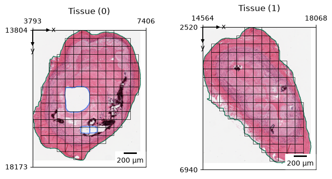
We can specify a name on the key_added parameter to save different tiling sizes and strategies on the same image. Note how the tiling is performed on the tissues we defined before.

The tiling result#

After tiling, LazySlide stores all tile information in a GeoDataFrame (by default named tiles).

Each tile is linked to its parent tissue through the tissue_id column, maintaining the hierarchical relationship between tissues and tiles. Let’s examine the tiles data:

wsi["tiles"]

	tile_id	tissue_id	geometry
0	0	0	POLYGON ((4052 16394, 4052 16653, 3793 16653, ...
1	1	0	POLYGON ((4052 16653, 4052 16912, 3793 16912, ...
2	2	0	POLYGON ((4311 15617, 4311 15876, 4052 15876, ...
3	3	0	POLYGON ((4311 15876, 4311 16135, 4052 16135, ...
4	4	0	POLYGON ((4311 16135, 4311 16394, 4052 16394, ...
...	...	...	...
248	248	1	POLYGON ((17672 5887, 17672 6146, 17413 6146, ...
249	249	1	POLYGON ((17672 6146, 17672 6405, 17413 6405, ...
250	250	1	POLYGON ((17672 6405, 17672 6664, 17413 6664, ...
251	251	1	POLYGON ((17931 5887, 17931 6146, 17672 6146, ...
252	252	1	POLYGON ((17931 6146, 17931 6405, 17672 6405, ...

253 rows × 3 columns

tiles can be visualized using the tiles function in plotting module.

zs.pl.tiles(wsi, tissue_id="all", linewidth=0.5)

../_images/624ff4b8de7daeb71274febf066a3f6806e41acd8b3ee5d13a561b488bf8cf15.png

Evaluating tile quality#

Just as we evaluated the quality of entire tissue regions earlier, we can also assess the quality of individual tiles. This is particularly important because not all tiles are equally informative or suitable for analysis. Some tiles might be:

Out of focus
Contain scanning artifacts
Have poor contrast
Contain mostly background or whitespace

LazySlide provides prediction models specifically designed for tiles. Let’s apply a QC model from pathprofiler:

zs.tl.tile_prediction(wsi, 'pathprofilerqc')

wsi["tiles"]

	tile_id	tissue_id	geometry	diagnostic_quality	visual_cleanliness	focus_issue	staining_issue	tissue_folding_present	misc_artifacts_present
0	0	0	POLYGON ((4052 16394, 4052 16653, 3793 16653, ...	0.212358	-0.052757	0.318834	0.267329	0.003896	0.743416
1	1	0	POLYGON ((4052 16653, 4052 16912, 3793 16912, ...	0.158073	-0.020617	0.272104	0.252748	-0.042276	0.838861
2	2	0	POLYGON ((4311 15617, 4311 15876, 4052 15876, ...	0.036068	-0.043858	0.180339	0.249886	0.013996	0.907113
3	3	0	POLYGON ((4311 15876, 4311 16135, 4052 16135, ...	0.087878	-0.023368	0.206672	0.204105	0.028838	0.832568
4	4	0	POLYGON ((4311 16135, 4311 16394, 4052 16394, ...	0.043891	-0.016791	0.156625	0.159387	0.010374	0.867012
...	...	...	...	...	...	...	...	...	...
248	248	1	POLYGON ((17672 5887, 17672 6146, 17413 6146, ...	0.246704	0.063703	0.077684	0.355271	0.022953	0.569547
249	249	1	POLYGON ((17672 6146, 17672 6405, 17413 6405, ...	-0.034062	0.002440	0.051641	0.194340	0.007238	0.886124
250	250	1	POLYGON ((17672 6405, 17672 6664, 17413 6664, ...	0.170865	0.018940	0.088636	0.259241	0.003885	0.737012
251	251	1	POLYGON ((17931 5887, 17931 6146, 17672 6146, ...	0.072131	-0.048144	0.175295	0.202928	0.005964	0.975038
252	252	1	POLYGON ((17931 6146, 17931 6405, 17672 6405, ...	0.001734	-0.024649	0.129624	0.177759	-0.023923	0.950272

253 rows × 9 columns

Visualizing tile quality scores#

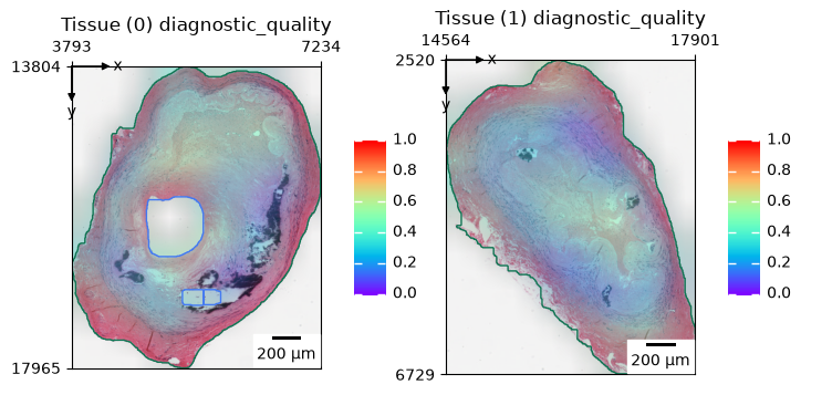
After calculating quality scores, it’s helpful to visualize them to identify patterns or problematic regions. LazySlide makes this easy by allowing you to color tiles based on any numerical property in the tiles dataframe.

Let’s visualize the contrast scores we just calculated:

zs.pl.tiles(wsi, tissue_id="all", color="diagnostic_quality", cmap="rainbow", 
            smooth=True, alpha=.5, vmin=0, vmax=1)

../_images/c4a47b024ba0edf80e8f27ea000b22a0f77df16bb0f7f96ec3c71408db9a6b51.png

Step 6: Feature extraction - transforming images into numerical representations#

We’ve now reached a crucial step in our preprocessing pipeline: feature extraction. This process transforms our image tiles into numerical representations (feature vectors) that capture the morphological characteristics of the tissue.

Why feature extraction matters#

Feature extraction is essential because:

It converts complex visual information into a format that machine learning algorithms can process
It enables quantitative comparison between different tissue regions
It forms the foundation for tasks like classification, clustering, and anomaly detection

Using vision models for feature extraction#

The most effective way to extract meaningful features from histology images is to use pre-trained vision models. These models, often trained on millions of images, have learned to recognize patterns and structures that are relevant to many visual tasks.

LazySlide supports a wide range of vision models:

Standard architectures from the timm library (ResNet, DenseNet, EfficientNet, etc.)
Specialized pathology foundation models
Custom models that you can provide

You can explore the available timm models with:

import timm
timm.list_models()

zs.tl.feature_extraction(wsi, "resnet50")

Using foundation models for pathology#

While general-purpose vision models like ResNet50 work well for many tasks, LazySlide also provides access to specialized foundation models that have been specifically trained on histology images. These models often capture pathology-specific features more effectively.

Let’s see what foundation models are available:

zs.models.list_models()[0:8]

['cytosyn', 'conch', 'medsiglip', 'musk', 'omiclip', 'plip', 'prism', 'titan']

Note

Some foundation models require access permissions from their creators. If you encounter an access error, you’ll need to:

Request access at the corresponding Hugging Face repository
Generate a token from your Hugging Face account
Login using the token

To run feature extraction on a foundation model:

zs.tl.feature_extraction(wsi, "uni2")

wsi

WSI: datasets--rendeirolab--lazyslide-data/snapshots/c455e26e8fbadada072d2ce348f563fa72c27eb6/GTEX-1117F-0526.svs
Reader: openslide
Dimensions: 19958×19919 (h×w), 3 Pyramids
Pixel physical size: 0.49 MPP (20X)

SpatialData object, with associated Zarr store: /home/runner/work/lazyslide-tutorials/lazyslide-tutorials/tutorials/datasets--rendeirolab--lazyslide-data/snapshots/c455e26e8fbadada072d2ce348f563fa72c27eb6/GTEX-1117F-0526.zarr
├── Images
│     └── 'wsi_thumbnail': DataArray[cyx] (3, 1996, 1992)
├── Shapes
│     ├── 'dl-tissues': GeoDataFrame shape: (2, 2) (2D shapes)
│     ├── 'tile_overlap_0.1': GeoDataFrame shape: (311, 3) (2D shapes)
│     ├── 'tile_stride_200': GeoDataFrame shape: (415, 3) (2D shapes)
│     ├── 'tiles': GeoDataFrame shape: (253, 9) (2D shapes)
│     └── 'tissues': GeoDataFrame shape: (2, 51) (2D shapes)
└── Tables
      └── 'resnet50_tiles': AnnData (253, 2048)
with coordinate systems:
    ▸ 'global', with elements:
        wsi_thumbnail (Images), dl-tissues (Shapes), tile_overlap_0.1 (Shapes), tile_stride_200 (Shapes), tiles (Shapes), tissues (Shapes)
with the following elements not in the Zarr store:
    ▸ tile_stride_200 (Shapes)
    ▸ resnet50_tiles (Tables)
    ▸ tiles (Shapes)
    ▸ tile_overlap_0.1 (Shapes)
    ▸ dl-tissues (Shapes)

Features are saved as AnnData store with a convention of “{model name}_{tiles key}”.

Feature aggregation basics#

When analyzing large datasets, it’s common practice to summarize the extracted features into a single 1D vector that represents each tile. This makes downstream analysis more efficient and interpretable.

LazySlide allows you to aggregate features at different levels. For example:

Tile-level aggregation (default): Each tile is represented by its own feature vector.
Tissue-level aggregation: By specifying by="tissue_id", you can pool features across all tiles belonging to the same tissue region, creating a summary vector for each tissue.

zs.tl.feature_aggregation(wsi, "resnet50")
zs.tl.feature_aggregation(wsi, "resnet50", by="tissue_id")

wsi["resnet50_tiles"]

AnnData object with n_obs × n_vars = 253 × 2048
    obs: 'tile_id', 'library_id'
    uns: 'spatialdata_attrs', 'agg_ops'
    varm: 'agg_slide', 'agg_tissue_id'

wsi.fetch.features_anndata("resnet50")

AnnData object with n_obs × n_vars = 253 × 2048
    obs: 'tile_id', 'tissue_id', 'diagnostic_quality', 'visual_cleanliness', 'focus_issue', 'staining_issue', 'tissue_folding_present', 'misc_artifacts_present'
    uns: 'tile_spec', 'slide_properties'
    obsm: 'spatial'
    varm: 'agg_slide', 'agg_tissue_id'

Save on the disk#

Now that we finished with our preprocessing. Remember to save the wsidata. By default it is saved side by side with the WSI. When you open the WSI next time, it will automatically pick up the wsidata.

wsi.write()

Notice that after saving, your SpatialData is now associated with a disk storage.

wsi

WSI: datasets--rendeirolab--lazyslide-data/snapshots/c455e26e8fbadada072d2ce348f563fa72c27eb6/GTEX-1117F-0526.svs
Reader: openslide
Dimensions: 19958×19919 (h×w), 3 Pyramids
Pixel physical size: 0.49 MPP (20X)

SpatialData object, with associated Zarr store: /home/runner/work/lazyslide-tutorials/lazyslide-tutorials/tutorials/datasets--rendeirolab--lazyslide-data/snapshots/c455e26e8fbadada072d2ce348f563fa72c27eb6/GTEX-1117F-0526.zarr
├── Images
│     └── 'wsi_thumbnail': DataArray[cyx] (3, 1996, 1992)
├── Shapes
│     ├── 'dl-tissues': GeoDataFrame shape: (2, 2) (2D shapes)
│     ├── 'tile_overlap_0.1': GeoDataFrame shape: (311, 3) (2D shapes)
│     ├── 'tile_stride_200': GeoDataFrame shape: (415, 3) (2D shapes)
│     ├── 'tiles': GeoDataFrame shape: (253, 9) (2D shapes)
│     └── 'tissues': GeoDataFrame shape: (2, 51) (2D shapes)
└── Tables
      └── 'resnet50_tiles': AnnData (253, 2048)
with coordinate systems:
    ▸ 'global', with elements:
        wsi_thumbnail (Images), dl-tissues (Shapes), tile_overlap_0.1 (Shapes), tile_stride_200 (Shapes), tiles (Shapes), tissues (Shapes)

You can always change where it should be saved

import tempfile

with tempfile.TemporaryDirectory() as tmp:
    store = f"{tmp}/temp.zarr"
    wsi.write(store)

    wsi = open_wsi(slide, store=store)

Preprocessing a WSI: From raw image to analysis-ready data

Contents

Preprocessing a WSI: From raw image to analysis-ready data#

Setting up environment#

Step 1: Opening a whole slide image#

Step 2: Understanding the WSIData object#

Step 3: Exploring WSIData object#

Slide Properties

Saving Our Work#

Step 4: Tissue Segmentation#

Examining the segmentation results#

Focusing on individual tissue pieces#

Don’t forget to save your work!#

Loading previously saved work#

Advanced topic: Deep learning-based tissue segmentation#

Calculating tissue properties#

Step 5: Tiling - Breaking down the WSI into manageable pieces#

Why tiling is essential#

Harmonization Across Slides#

LazySlide’s flexible tiling capabilities#

Creating overlapping tiles#

The tiling result#

Evaluating tile quality#

Visualizing tile quality scores#

Step 6: Feature extraction - transforming images into numerical representations#

Why feature extraction matters#

Using vision models for feature extraction#

Using foundation models for pathology#

Feature aggregation basics#

Save on the disk#